LO-SL BRDF Explained... (Part 2)

Time fly so fast... wheew. I've been so busy this month but as I have promised, here's the continuation of the LO-SL BRDF. Much thanks to Alberto Demichelis for giving me this challenging task even with some heated discussions along the way, but all for the sake of pointing me to the right direction.

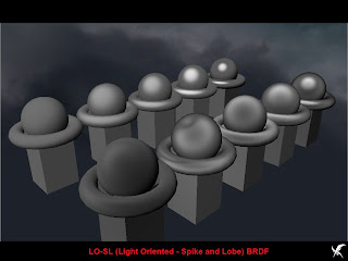
The screenshot above is a material test running on our pipeline. I removed the ambient light and turned off any AO or postprocesses so its easier to see their light response. Currently, these are just directional diffuse+specularity as our requirement does not need realtime reflection so far. All of the objects are RGB(128,128,128) meaning real gray to purposely visualize the high, mid and low tone light response. The light is directional light with a white color RGB(255, 255, 255). The further 4 materials are actually simulating Blinn-Phong lighting model having the specularity size differences and some factor to simulate roughness. The nearer 4 materials are metals, (at least I tried to mimic). Starting from the left is rough iron, brushed metal (notice some anisotropic effect to it), copper, gold and chrome. Ofcourse, the effect will be much visible once normal mapping is applied to them.

What is Light Oriented-Spike and Lobe BRDF? It is a modified-simplified approach of the Bidirectional Reflectance Distribution Function so much so that it can be use for realtime-game application. It is not however, an exact math replacement of the full Oren-Nayer reflection model. Its goal is not to be precise but rather to just be convincing enough. In researching about photometry, I found out that there are different ways in gathering reflectance distribution data of different materials. Some plot the reflectance into a 3D or volume data. LO-SL BRDF simplify this volume of data by mimicking the values into 'strategicly aligned' 1D waves along the Normal (no tangents needed). This waves are then stored into a lookup table shrinking its math into a simple texture sample. The beauty of this is that, in possible future implementation this can be extended to doing away with waves and instead use curves or vector data for better plotting precision before they are save in the look-up table texture.

Here is a screenshot of the look-up generator for the LO-SL BRDF...

You'll notice in the right part of the screenshot are 4 groups of control values. Theta Incident, Theta Reflectance, Phi Incident+Reflectance and Specularity. Right now, the Specularity part is an anomaly in my implementation. I still have to research the actual relation of specularity in my implementation. (I'll be delighted if anyone can help me with this or even to point me to the right direction). You may also notice that it only deals with monochromatic distortions. Currently, this is only our requirement so we decided to only use monochromatic. Of course, tri-color distortion (meaning individual/independent distortions of RGB colors), example reflectance of bubbles or oil sheen in water, can still be implemented by storing 3 channels per angle. Plus we are saving the remaining channels for something special....a 'SS' special. (*wink**wink*). Each of these control values (except Specularity) represents the 1D wave slicing the full BRDF into 3 1D waves.

The control values are...

Theta θ - represents the angle with highest spike or the peak of the wave

dθ - is the differential angle or range/size/cone angle of the lobe

C. Pow - is a pow function to steepen the curve

Factor - is the wave magnitude factor

You can also notice that the left part of the of screenshot are composed of 4 viewports. The upper left, is the preview. The rest are each channel of the look-up table. The upper right is the look-up table preview of  the Theta Incident and Theta Reflectance 'combined' together (will  be explained later). The lower left is the Phi Incident+Reflectance combined with Specularity. This one I'm still not convinced if my assumptions are correct on this. Previously, I separated the Phi I+R and Specularity as they are not possible to combine. So before they were in the lower left and lower right.

Combining these waves into a single 2D channel is possible due to its one important commonality... the Normal. The T or time of the wave/curve is Normal 0 to 1 (actual represents -1 to 1 of the Normal). Another relation is 'multiplication', so each of the result of the 1D wave are eventually multiplied together, hence we can pre-multiply it.

I know its quite confusing. I guess I'm not really good translating this into words. I need some sort of illustration for this. Anyway, to those who are still with me, here's the formula,

Theta Incident = N.L

Theta Reflectance = N.V

Phi Incident+Reflectance = V.(normalize(N-L))

Specularity = N.H (I'm still not sure to keep this)

Maybe in the future I can produce a study papers on this. Or maybe someone wants to offer me to write an article for their awesome highly anticipated graphics book. Yes? No? No takers? Oh well. hehhehe...